
Arjhun S
@arjuns0206Hamilton, Will, Zhitao Ying, and Jure Leskovec. “Inductive representation learning on large graphs.” Advances in neural information processing systems 30 (2017).
 https://snap.stanford.edu/graphsage/
I attempt to demystify this paper in this article by making it as simple as possible. The paper associated with this article can be found here.
A quick background on GCNs (skip if you already know)
A graph **G **is represented as:
where:
-
**V **is the set of nodes (vertices) with |V| = N nodes
-
E is the set of edges, which define relationships between nodes.
Now that we know what a graph is, let’s talk about how GCNs process the data that we get from a graph.
The key idea in a GCN is message passing, where each node updates its feature representations by aggregating information from its neighbours. This is under the assumption that there is an edge between two nodes for a reason and this relationship should contribute to the overall task that we would like the GCN to perform.
At each layer k, the node features for any given node, is updated using the neighbouring nodes’ features. The step (also known as the Graph Convolutional step) looks like this:
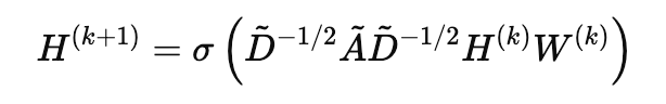
where:
-
H^(k) = node feature matrix at layer k.
-
W^(k) = learnable weight matrix.
-
Acap = A + I is the adjacency matrix with self-loops (I is the identity matrix).
-
Dcap is the diagonal degree matrix, where each diagonal element ᵢᵢ represents the degree of the nodeᵢ.
-
σ is an activation function.
The intuition behind this step is to propagate and transform node features across the graph in a way that incorporates both the node’s own features and that of its neighbours. The term D^-1/2 * A * D^-1/2 normalises the adjacency matrix A (which includes self-loops) using the degree matrix D, ensuring that the influence of each neighbour is appropriately weighted.
GraphSAGE
Intuition
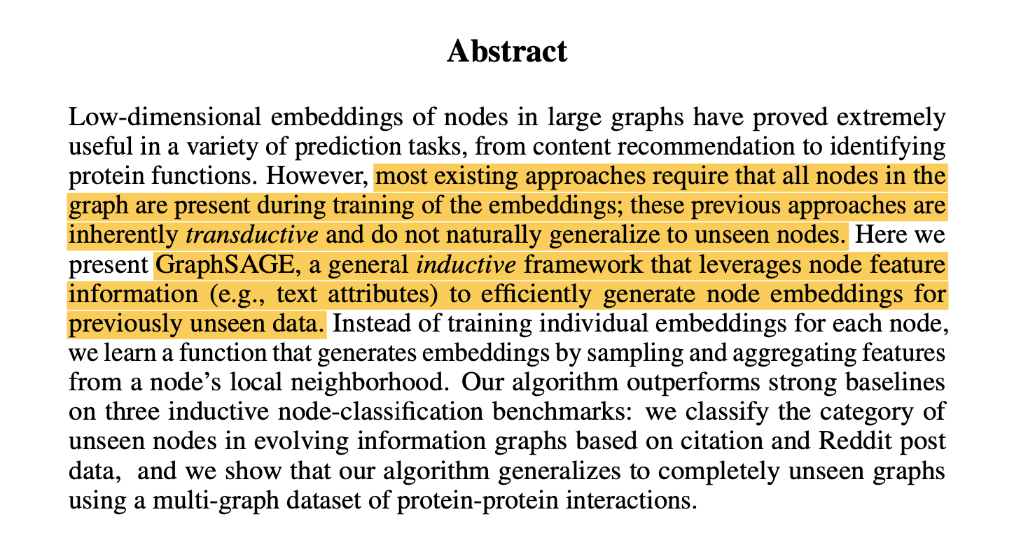 Inductive Representation Learning on Large Graphs
If you read the highlighted text carefully, you understand what they are trying to do differently. The existing GCN uses the entire Adjacency matrix A to aggregate node features, which makes it transductive. However, GraphSAGE wants to use an inductive framework to generalise well on unseen data. Let’s see how exactly they achieve that.
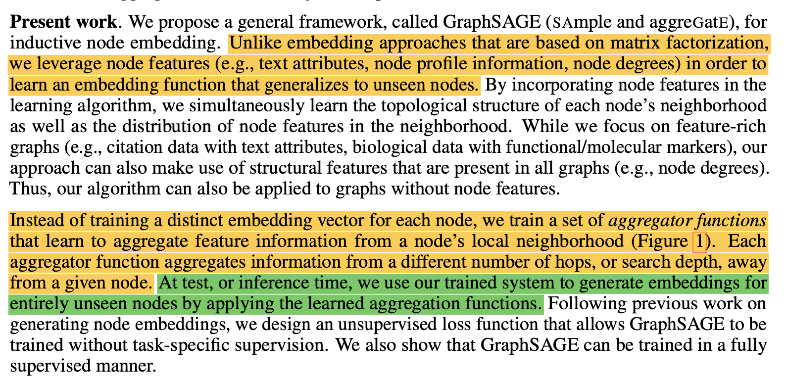
They claim that they use aggregator functions that learn the node’s feature information from its local neighbourhood. This trained aggregation function, is designed to be able to be used on unseen nodes. This means, we don’t really need the entire graph to compute a single node’s feature representations at a given layer.
You may argue that we might lose some critical information by resorting to the local neighbourhood information in calculating the node features. We will get back to this later.
Let’s look at how they achieve this through the algorithm mentioned in their paper. I have clipped it to focus on the important parts.
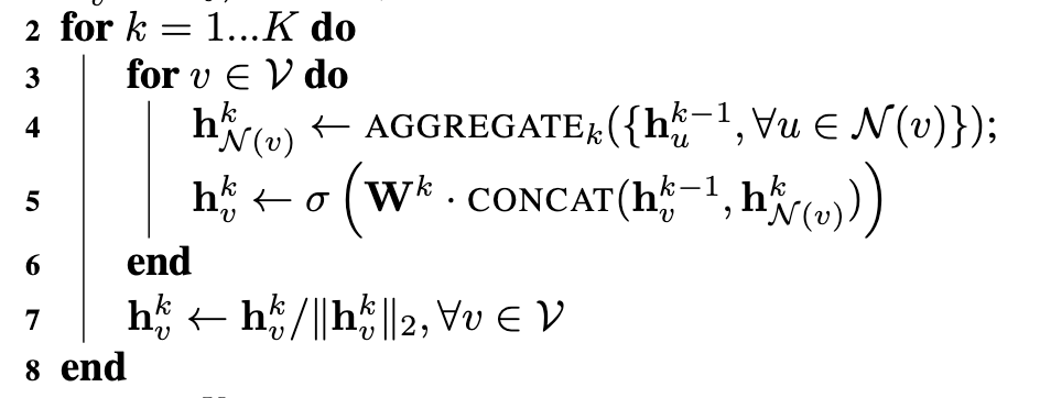
Here K represents the depth of the network, V represents the vertices and N represents the neighbourhood function of a given vertex v. At each layer, for each of the vertices (nodes), we first execute the aggregation function that calculates node features of v using its neighbours (more on aggregation functions later). Then we proceed to do a concat operation of the currently calculated node features using the aggregation function based on the neighbours and the existing node features of vertex v.
why concat?
This is a very important step of GraphSAGE. Why do we need to concat? Intuitively, it’s because we don’t want the neighbour information to overwhelm the node features. We can take social media posts and comments as an example. If a social media post is the vertex in this case, and the comments are the neighbourhood nodes, we don’t want the features of the neighbours to take over the features of the post. Hence instead of simply reassigning, we concat.
Once we concat, it’s passed through a fully-connected layer and non-linearity.
According to the writers of the paper:
 Intuition
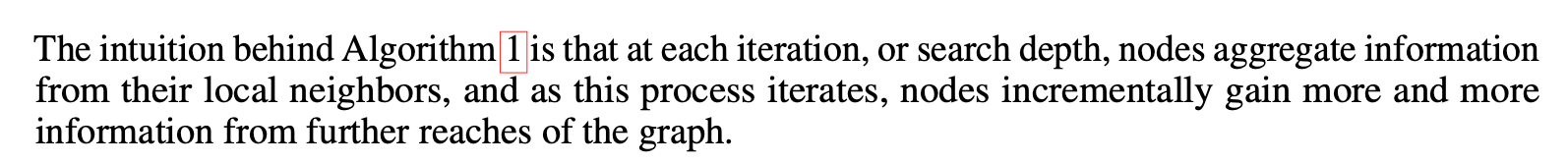
This is how GraphSAGE argues that nodes incrementally gain more and more information from further reaches of the graph.
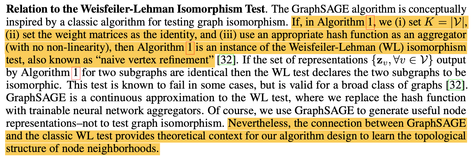
Connection to the Weisfeiler-Lehman Graph Isomorphism Test (Skip if not interested)
 Weisfeiler-Lehman
Weisfeiler-Lehman’s graph isomorphism algorithm is considered state-of-the-art in Graph comparison techniques. It works by iteratively hashing node labels based on their neighbours’ labels. This refinement continues for K iterations If two graphs have the same set of final node labels, they are declared isomorphic.
Now let’s see how this compares to GraphSAGE. We start with an initial feature vector for each node (or vertex). At each step, we aggregate information from the local neighbourhood. Instead of discrete labels, we have a trainable weight matrix and non-linearities and after K layers, we use this learned information to do tasks like clustering or classification.
Loss function for unsupervised learning
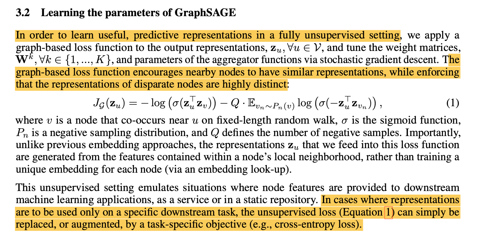
The paper proposes a loss function to be used with GraphSAGE in an unsupervised setting.
Let’s clearly look at what the loss function is trying to achieve. The underlying idea is the maximise similarity between node representations of nodes that co-occur together (nodes in the same neighbourhood during a random-walk) and minimise the similarity of nodes that do not co-occur together (negative sampling). The first and second terms in the loss equation target the former and latter respectively.
The first term
The dot product of the representations of any 2 given nodes is the cosine similarity term. The sigmoid function is used to squash the output from the dot product (which ranges from -1 to 1) into a 0–1 range. The negative log penalises values close to 0 by being largely negative.
The second term
In contrast to a random-walk, negative sampling aims to create dissimilar pairs. We take the same log term, but this time there is a negative sign after the dot product, which is going reverse penalise (minimise similarity), over *Q *negative samples.
Aggregation functions proposed
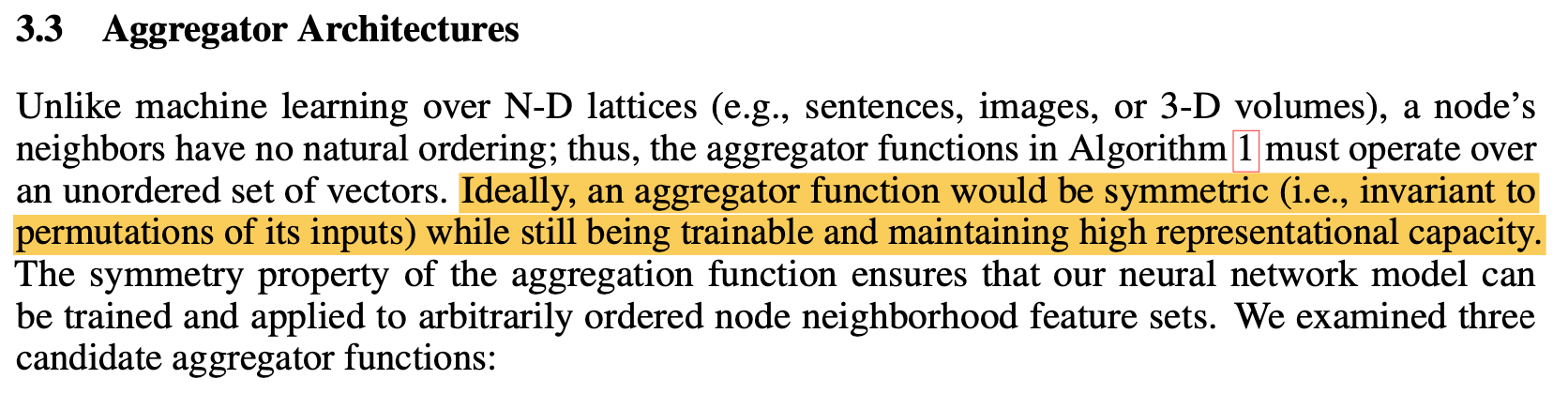
To put in simple words, the neighbours of a given node are unordered. It could be both {v1, v2, v3} or {v2, v1, v3} and they mean the same thing in this context. They expect an aggregation function to output the same result regardless of the order of neighbourhood nodes.
Mean Aggregator
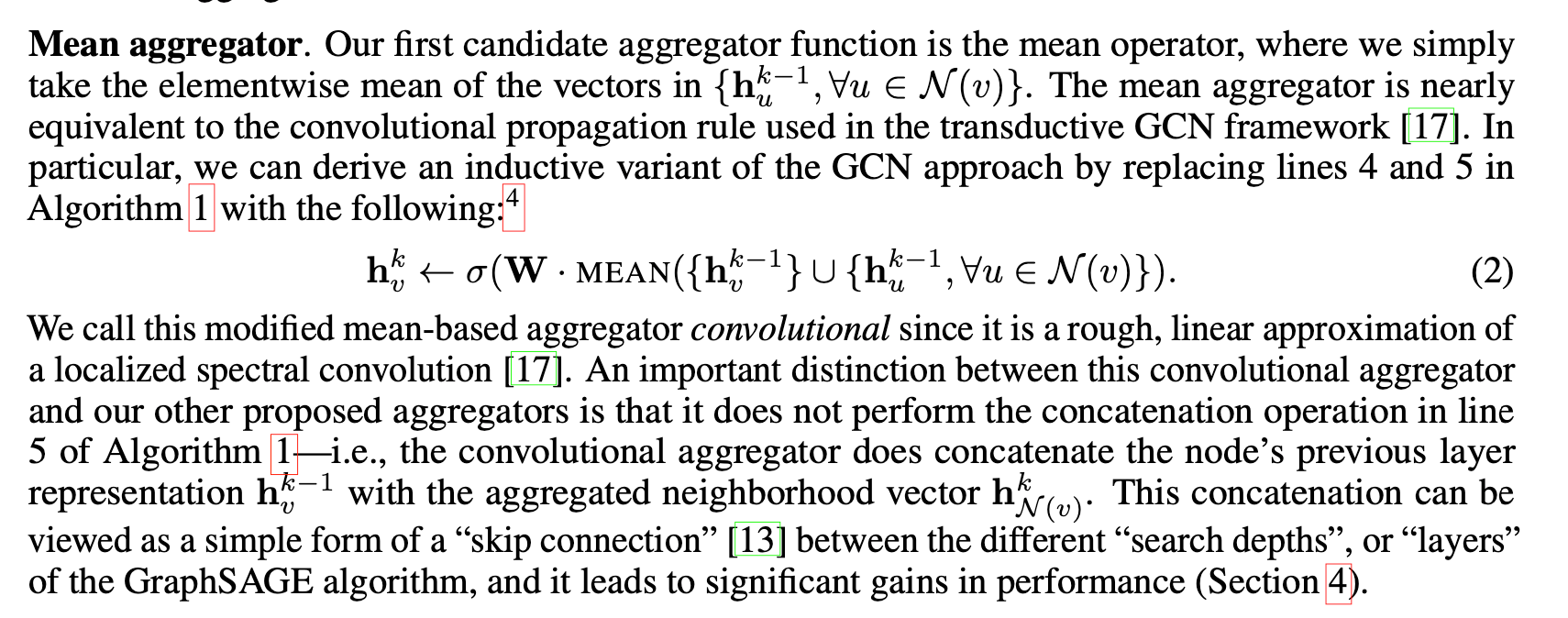
The mean aggregator is referred to be nearly equivalent (or the inductive variant) to the convolutional propagation rule used in the GCN framework. This is because of how we only apply the aggregation function to a given set of local neighbours, unlike how a GCN operation considers the entire neighbour set normalised by the degree.
The writers here mention that the concatenation does not happen for mean aggregation. However, in the torch implementation of GraphSAGE, it does perform the concat operation, regardless of the aggregators chosen. It is also mentioned that the concat operation improves performance. I leave this specific interpretation to the reader.
LSTM Aggregator
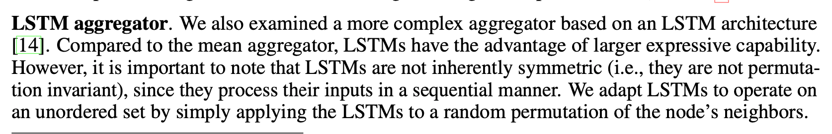
I am not going to go in-depth into LSTM (Long-short-term-memory) in this article, but, to put it simply, they are an RNN architecture that is designed to process sequential data by maintaining memory of previous inputs (time steps). You can read more about LSTM here.
This nature of LSTMs being sensitive to sequence makes them asymmetric. The writers simply ignore this and have given a random permutation of neighbours to the LSTM.
In essence, LSTMs are known for their ability to capture long-range dependencies and context, and hence have been used as a candidate aggregator function.
Pooling Aggregator
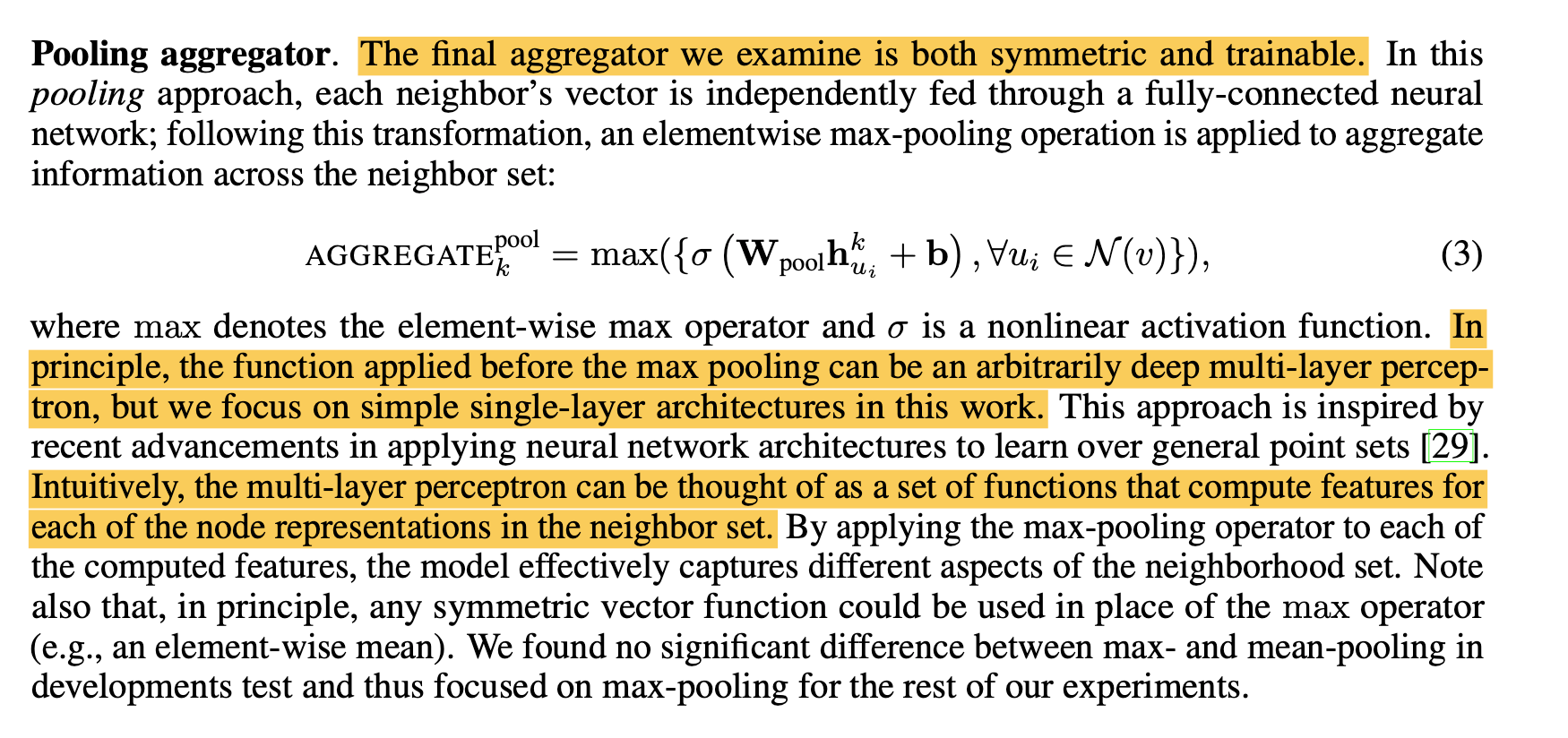
The pooling aggregator works slightly differently. Unlike the other 2 aggregators, they don’t directly operate on the node features of the neighbourhood nodes. Instead, there is a fully connected layer that has trainable weights which operate on the node features. This fully connected MLP could be indefinitely large depending on requirements, and a max pooling operation is done on the vectors resulting from the outputs of the MLP, essentially capturing different aspects of the neighbourhood set.
I am choosing not to cover the specific test results mentioned in the paper, which anyone can browse through. The link to the paper can be found at the beginning of the article.
Conclusion
That’s it folks! I hope this article helped you understand this manuscript and the architecture proposed, which has been extremely successful in a lot of network research (including one of mine). You can find the in-built torch implementation of this model here.
Thanks for reading through. Cheers.